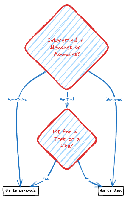
Assume that you're a traveller planning your next weekend getaway and have two amazing options: A relaxing beach trip to Goa or a thrilling mountain adventure in Lonavala. But, how do you decide one way or the other? This is where Decision Trees come in. They are like flowcharts, visually representing all the scenarios. Let's look deeper into this example.

Our first question would be if the person is interested in beaches or mountains. Another decisive question could be if the person is fit for a trek or a hike.

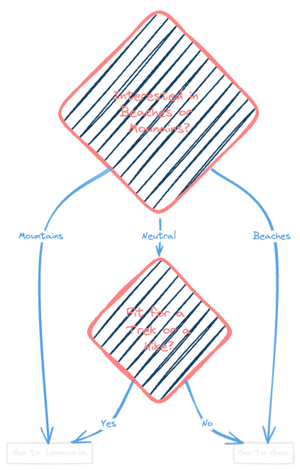
Let's look at a visual representation of how a Decision Tree could help in this.

Shown above is a standard representation of a hypothetical situation but there's a lot of math that goes into it. Ready for it? Let's get right in!

Decision Tree Variants

The decision tree is not restricted to just classification or regression. There is a separate arithmetic calculation in each node for each of these variants. The variants are:

• Decision Tree Classifier
• Decision Tree Regressor

The Decision Tree evaluates each given feature to find the most relevant one and equates the results for that specific feature first. This is done until all the features are evaluated and the leaf node is encountered. A leaf node is defined as a node to which there are no Childs. This node is used for prediction. As for the tuning, the depth of the decision tree could be restricted, meaning that longest path between the root node and a leaf node is restricted to a specified number.

Decision Tree Classifier

The decision tree classifier is very similar to a flow chart. Each node of decision tree has certain evaluations that go into it. There are two different ways to do this. One is Information Gain method, and the other is Gini Index method. Let's look at the steps involved in building these and the Mathematics and Statistics behind it.

Decision Tree Classifier: Information Gain Method

Step 1: Calculate the Entropy of entire Dataset

Entropy is defined as randomness or uncertainty in the given data or situation. First step in building the decision tree classifier is to calculate the entropy of the entire dataset. This can be done by calculating the entropy of the label or the target column. The formula for this is:

Step 2: Calculate Entropy of each Feature Column

When calculating entropy of each feature column, we need to first calculate entropy for each unique value in the selected feature column using the following equation. Select all the rows corresponding to selected value and calculate entropy with respect to those rows.

After calculating the entropy for each unique value in the feature column, next step is to calculate the entropy of the feature column using the following arithmetic equation:

Repeat this process for each feature column.

Step 3: Information Gain Index

Information Gain is a measure used to determine which feature column is to be selected next.

The value with highest Information Gain is selected to be the root node or the next node.

Working Example

Now let's look at how this works in practice. Consider the following dataset:

The Entropy of the entire dataset is:

Next step is to calculate Entropy for each feature column.

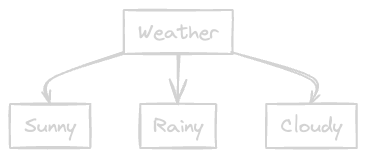
• For Weather: There are three unique values: Sunny, Rainy and Cloudy

• For Temperature: There are three unique values: Hot, Cool and Mild

• For Humidity: There are two unique values: High and Normal

• For wind: There are two unique values: Weak and Strong

Now that we have all the Information Gain Index, let's analyze them.

The highest Information Gain is to be selected as root node. In this case, it is Weather. Hence, the decision tree we get now is:

Now let's do the further processing for the "Sunny" Condition. Consider the following dataset:

• For Temperature: There are three values: Hot, Mild, Cool

• For Humidity: There are two values: High and Normal

• For Wind: There are two values: Weak and Strong

Let's check all the Information Gain Indexes:

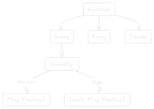
Since the highest is Humidity, the Humidity node comes after Sunny.

From the dataset, we can clearly notice that when Humidity is high, football is not played and when it is normal, football is played. Hence we can insert a leaf node or output node for this.

The resulting decision tree is as follows:

Now let's check the data for Rainy:

• For Temperature: There are two values: Mild, Cool

• For Humidity: There are two values: High and Normal

• For Wind: There are two values: Weak and Strong

Let's check all the Information Gain Indexes:

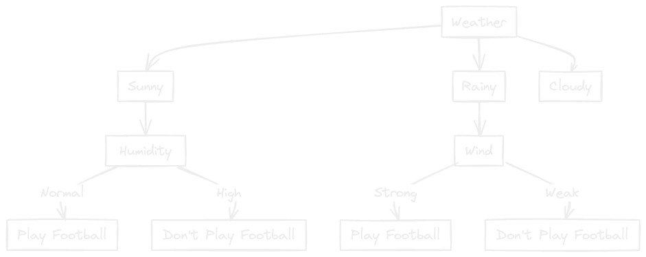
Since the highest is Wind, the Wind node comes after Rainy.

It can be seen that when Wind is Strong, football is not played and when it is Weak, football is played. Hence we can insert a leaf node or output node for this.

The resulting decision tree is as follows:

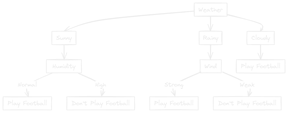
Now let's look at the data for cloudy weather!

We can see that all the labels are "Yes" in this data. Hence we can conclude that for cloudy weather, football will be played regardless of temperature, humidity and wind.

The final decision tree constructed will be as follows:

Decision Tree Classifier: Gini Index Method

Gini index is very similar to Information Gain Index. Here are the equations and steps with respect to Gini-Index Method. Gini Index is a more powerful measure of entropy in datasets and is hence proven to be more effective than Information Gain.

Step 1: Calculate Gini-Index of each Feature Column

After calculating the entropy for each unique value in the feature column, next step is to calculate the entropy of the feature column using the following arithmetic equation:

Repeat this process for each feature column.

Step 2: Select the Attribute with Lowest Gini-Index as Decision Node

The feature with lowest gini-index is utilized as the decision node and the process is repeated until leaf node is achieved.

Working Example

Consider the following data:

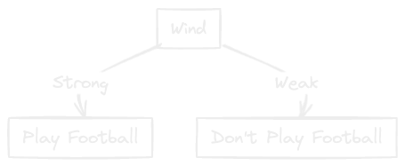
• For Temperature: There are 3 values: Hot, Mild and Cool

• For Humidity: There are two values: High and Normal

• For Wind: There are two values: Weak and Strong

The lowest Gini Index is of Humidity. Therefore Humidity is selected as decision node.

Therefore the tree that is formed is:

Python Implementation of Decision Tree Classifier

Following is the Python code for decision tree classifier:

			# Import Required Modules
from sklearn.tree import DecisionTreeClassifier
from sklearn import tree
from sklearn.metrics import confusion_matrix, ConfusionMatrixDisplay
import pandas as pd
import matplotlib.pyplot as plt
 
# Data Reading Pre-Processing
data = pd.read_excel("data.xlsx")
data['Weather'].replace(['Sunny','Rainy','Cloudy'], [0,1,2], inplace=True)
data['Temperature'].replace(['Hot','Cool','Mild'], [0,1,2], inplace=True)
data['Humidity'].replace(['High','Normal'], [0,1], inplace=True)
data['Wind'].replace(['Weak','Strong'], [0,1], inplace=True)
data['Play Football'].replace(['No','Yes'], [0,1], inplace=True)
 
# Separating Features and Label
x = data.drop("Play Football", axis=1)
y = data[["Play Football"]]
 
# Model Training
model = DecisionTreeClassifier()
model.fit(x, y)
 
# Confusion Matrix
cm = confusion_matrix(y, model.predict(x))
ConfusionMatrixDisplay(cm).plot()
 
# Append predicted values to data to display
data = pd.read_excel("data.xlsx")
data["Model Predictions"] = model.predict(x)
data['Model Predictions'].replace([0,1], ["No","Yes"], inplace=True)
	

			# Import Required Modules
from sklearn.tree import DecisionTreeClassifier
from sklearn import tree
from sklearn.metrics import confusion_matrix, ConfusionMatrixDisplay
import pandas as pd
import matplotlib.pyplot as plt
 
# Data Reading Pre-Processing
data = pd.read_excel("data.xlsx")
data['Weather'].replace(['Sunny','Rainy','Cloudy'], [0,1,2], inplace=True)
data['Temperature'].replace(['Hot','Cool','Mild'], [0,1,2], inplace=True)
data['Humidity'].replace(['High','Normal'], [0,1], inplace=True)
data['Wind'].replace(['Weak','Strong'], [0,1], inplace=True)
data['Play Football'].replace(['No','Yes'], [0,1], inplace=True)
 
# Separating Features and Label
x = data.drop("Play Football", axis=1)
y = data[["Play Football"]]
 
# Model Training
model = DecisionTreeClassifier()
model.fit(x, y)
 
# Confusion Matrix
cm = confusion_matrix(y, model.predict(x))
ConfusionMatrixDisplay(cm).plot()
 
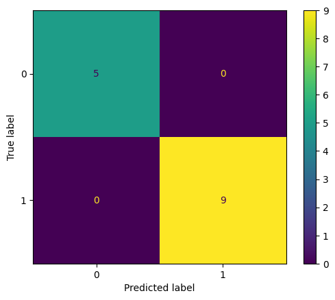
# Append predicted values to data to display
data = pd.read_excel("data.xlsx")
data["Model Predictions"] = model.predict(x)
data['Model Predictions'].replace([0,1], ["No","Yes"], inplace=True)
	

The Confusion Matrix produced by this code is as follows:

Confusion Matrix

It can be interpreted by this confusion matrix that all the predictions were accurate and there were 5 true negatives and 9 true positives.

This is all about the Decision Tree Classifier. If you have any questions regarding this, feel free to contact me.

Up next, we have the Decision Tree Regressor where we train the Decision Tree Algorithm to work with continuous values. Stay Tuned!