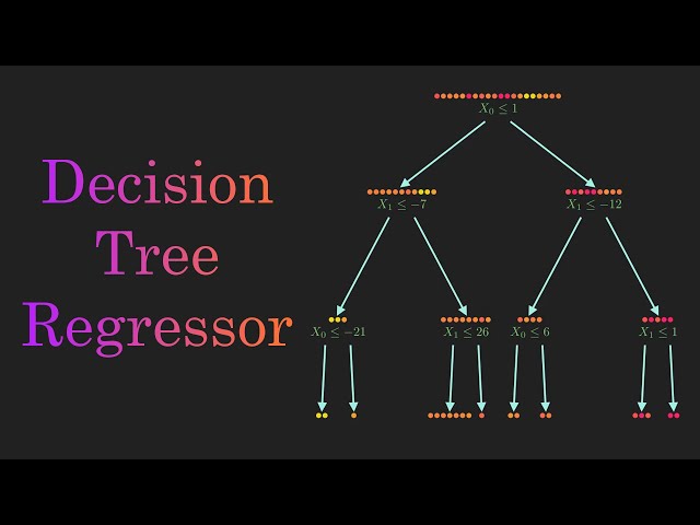
Decision Tree Regressor: A Branching Algorithm for Continuous Values
January 29, 2024

In our previous post, we dived into the world of Decision Tree Classification, uncovering its nuances and applications. Now, in this second part of our series, we're switching gears to explore Decision Tree Regression.
While Decision Tree Regression shares similarities with its classification counterpart, it's tailored to handle a different set of challenges—specifically, predicting continuous values. In this article, we'll unravel the inner workings of Decision Tree Regression, demystifying its approach, discussing its intuition, and delving into the mathematical concepts that drive its predictive power.
Intuition behind Decision Tree Regression
So, what's Decision Tree Regression all about? Well, it's a technique used for predicting continuous values. Imagine you have a bunch of data points with features like age, income, and education, and you want to predict something like house prices or stock prices. That's where Decision Tree Regression comes in handy.
Here's how it works: The algorithm starts by looking at all the data and figuring out which feature is the best to split the dataset on. It does this by trying different splits and choosing the one that reduces the variance of the target variable the most. This process continues, with the algorithm creating a tree-like structure until it decides it's time to stop, maybe when it reaches a certain depth or when there are too few data points left in a group.
Once the tree is built, making predictions is pretty straightforward. You start at the top of the tree with your new data and follow the branches based on its features until you reach a leaf node. At that point, the algorithm gives you the predicted value for your continuous variable.
The cool thing about Decision Tree Regression is that it can capture complex relationships between your features and your target variable. It's like creating a roadmap that can navigate through the twists and turns of your data to give you a good prediction.
There's some math involved too, of course. The algorithm uses measures like the Gini index or entropy to figure out the best splits and minimize errors. It's all about finding the best way to carve up your data so you can make the most accurate predictions.
Methodology
let's consider this small dataset with X and Y where Y is our target variable
| X | Y |
|---|---|
| 1 | 450 |
| 2 | 500 |
| 3 | 550 |
| 4 | 600 |
| 5 | 650 |
| 6 | 700 |
| 7 | 750 |
| 8 | 800 |
| 9 | 850 |
| 10 | 900 |
| 11 | 950 |
| 12 | 1000 |
| 13 | 1050 |
| 14 | 1100 |
| 15 | 1150 |
Now, let's build a simple Decision Tree Regression model using this dataset.
Building the Decision Tree
We'll start by building a decision tree with a single split based on the X value. We'll use the mean squared error (MSE) as the criterion for splitting.
1. Calculate the mean of Y:
2. Calculate the MSE for each split
Split at
- Calculate the mean of for , denoted by
- Calculate the MSE for this split, denoted as MSE
Split at
- Calculate the mean of for , denoted by
- Calculate the MSE for this split, denoted as MSE
3. Choosing the right split
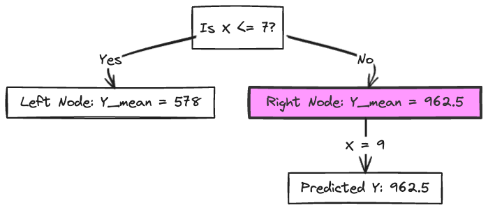
In this case, we would choose the split with the lowest MSE, which is the split at with


4. Predictions
Let's consider a sample unknown point with X = 9. Based on our decision tree, we can predict the value of Y for this point by following the splits in the tree.
Start at the root node: Since X = 9, we follow the right branch (X > 7).
Move to the right node: The mean of Y for this node () is 962.5.
Predicted Y: Based on the decision tree, our predicted value of Y for X = 9 is 962.5. Therefore, according to our decision tree model, for an unknown point with X = 9, we predict Y to be approximately 962.5.
This prediction is based on the splits and mean values obtained from our decision tree model.
Python Implementation
			from sklearn.tree import DecisionTreeRegressor
import numpy as np

# Sample dataset
X = np.array([1, 2, 3, 4, 5, 6, 7, 8, 9, 10, 11, 12, 13, 14, 15]).reshape(-1, 1)
y = np.array([450, 500, 550, 600, 650, 700, 750, 800, 850, 900, 950, 1000, 1050, 1100, 1150])

# Create and fit the decision tree regression model
model = DecisionTreeRegressor(random_state=42)
model.fit(X, y)

X_unknown = np.array([[9]])
predicted_y = model.predict(X_unknown)

print(f"The predicted value of Y for X = 9 is: {predicted_y[0]}")
The output would be
The predicted value of Y for X = 9 is: 850.0
The predicted value of Y for X = 9 is: 850.0
When you run this code, it should output the predicted value of Y for the unknown point X = 9 based on the decision tree regression model, using the optimal split points determined by the algorithm. The algorithm considers factors such as the feature that provides the best split, often using metrics like information gain or Gini impurity for classification problems, and variance reduction for regression problems.
if you look at the flow chart for this,

So this is all about Decision tree Regression in a nutshell. Meet you in the next post.
In this net post, we will see random forest and how it's different from Decision tree.