Three Musketeers of Gradient Descent

Gradient Descent

Machine Learning

# 4

January 17, 2024

S H

Shayaan Hussain

The gradient descent algorithm is mainly implemented in three variants:

Stochastic Gradient Descent
Batch Gradient Descent
Mini-Batch Gradient Descent

Each variant has its own benefits and produce their own results which are not necessarily the same. The main difference between these implementations is the amount of data that is utilized before calculating the gradient. Let's discuss each of these in more detail.

To study each of these variants, we will use the following data:

X	Y
1	8
6	33
9	48
5	28

To achieve y from x, the equation that will be used is:

y = mx + b

We have to optimize m and b to achieve the right 'y' value. For this purpose, we find the derivative equation of the cost function i.e. MSE in this case.

MSE = (y - (mx + b)) ^ 2

Differentiate MSE with respect to $m$ :

rac{d}{dm}MSE = -1(y - (mx + b))x

Differentiate MSE with respect to $b$ :

rac{d}{db}MSE = -1(y - (mx + b))

Now let us discuss each variant and their implementation for the above data.

Stochastic Gradient Descent (SGD)

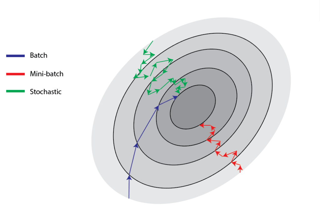
The SGD takes one sample at a time from the dataset and calculates the gradient based on that. It's like taking a peek down the hill and taking one small step at a time. This makes SGD fast and efficient for larger datasets but the output may be a bit noisy and zig-zag around the maze, making it inconsistent in some cases. SGD is suitable for applications like spam email detection.

Let's have a look at the code for Stochastic Gradient Descent:

			# Import required modules
import pandas as pd
import numpy as np
import matplotlib.pyplot as plt
import imageio
import os
plt.grid()
 
def derivative(x, y, m, b): # Function to caluclate derivatives
    m_derivative = -1 * (y - m * x - b) * x
    b_derivative = -1 * (y - m * x - b)
    return m_derivative, b_derivative
 
# Read the data
data = pd.read_csv("data.csv")
 
# Initialize parameters
m = np.random.uniform(-5, 5)
b = np.random.uniform(-5, 5)
learning_rate = 0.05
iterations = 100
 
rmse = [] # List to store RMSE values after each iteration
 
for iter in range(iterations): # Loop to count epochs
 
    for i in range(data.shape[0]): # Loop to iterate through data points
        
        # Calculate derivatives
        m_grad, b_grad = derivative(data["x"][i], data["y"][i], m, b)
        
        # Calculate Step Length
        m_step = learning_rate * m_grad
        b_step = learning_rate * b_grad
 
        # Update m and b value
        m = m - m_step
        b = b - b_step
    
    # Calculate RMSE Value
    rmse_temp = 0
    for i in range(data.shape[0]):
        rmse_temp += ((data["y"][i] - (m * data["x"][i] + b)) ** 2) ** 0.5
    rmse.append(rmse_temp / data.shape[0])
    
    # Plot RMSE value
    plt.plot(range(1, len(rmse) + 1), rmse, color='red')
    plt.xlim(0, 100)
    plt.ylim(0, 15)
    plt.xlabel('epochs')
    plt.ylabel('RMSE')
    plt.savefig(f"sgd_graphs/sgd_{iter}.png")
 
print(f"Achieved values : m = {np.round(m, 2)}, b = {np.round(b, 2)}") # Print achieved values
 
# GIF Generation
images = [imageio.imread(f"sgd_graphs/sgd_{x}.png") for x in range(len(os.listdir("sgd_graphs")))]
imageio.mimsave("sgd.gif", images)

			# Import required modules
import pandas as pd
import numpy as np
import matplotlib.pyplot as plt
import imageio
import os
plt.grid()
 
def derivative(x, y, m, b): # Function to caluclate derivatives
    m_derivative = -1 * (y - m * x - b) * x
    b_derivative = -1 * (y - m * x - b)
    return m_derivative, b_derivative
 
# Read the data
data = pd.read_csv("data.csv")
 
# Initialize parameters
m = np.random.uniform(-5, 5)
b = np.random.uniform(-5, 5)
learning_rate = 0.05
iterations = 100
 
rmse = [] # List to store RMSE values after each iteration
 
for iter in range(iterations): # Loop to count epochs
 
    for i in range(data.shape[0]): # Loop to iterate through data points
        
        # Calculate derivatives
        m_grad, b_grad = derivative(data["x"][i], data["y"][i], m, b)
        
        # Calculate Step Length
        m_step = learning_rate * m_grad
        b_step = learning_rate * b_grad
 
        # Update m and b value
        m = m - m_step
        b = b - b_step
    
    # Calculate RMSE Value
    rmse_temp = 0
    for i in range(data.shape[0]):
        rmse_temp += ((data["y"][i] - (m * data["x"][i] + b)) ** 2) ** 0.5
    rmse.append(rmse_temp / data.shape[0])
    
    # Plot RMSE value
    plt.plot(range(1, len(rmse) + 1), rmse, color='red')
    plt.xlim(0, 100)
    plt.ylim(0, 15)
    plt.xlabel('epochs')
    plt.ylabel('RMSE')
    plt.savefig(f"sgd_graphs/sgd_{iter}.png")
 
print(f"Achieved values : m = {np.round(m, 2)}, b = {np.round(b, 2)}") # Print achieved values
 
# GIF Generation
images = [imageio.imread(f"sgd_graphs/sgd_{x}.png") for x in range(len(os.listdir("sgd_graphs")))]
imageio.mimsave("sgd.gif", images)

The above code generates a demonstration of how SGD reduces the error or cost function value.

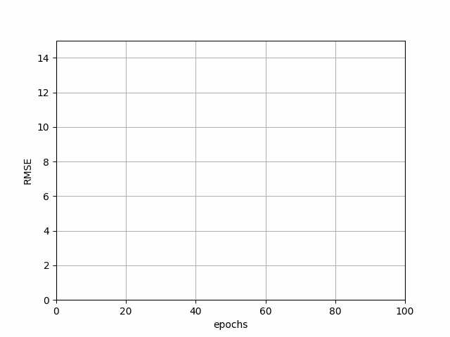
SGD Progression

Batch Gradient Descent (BGD)

The BGD takes in account all the data points while calculating the gradient. It's like taking a survey of a whole region before making a single, deliberate step. This definitely improves the performance of the algorithm, but the time complexity of this algorithm is way too high and it takes massive amount of time for larger datasets. That's where MBGD comes into play!

The code for BGD is as follows:

			# Import required modules
import pandas as pd
import numpy as np
import matplotlib.pyplot as plt
import imageio
import os
plt.grid()
 
def derivative(x, y, m, b): # Function to calculate derivatives
    m_derivative = -1 * (y - m * x - b) * x
    b_derivative = -1 * (y - m * x - b)
    return m_derivative, b_derivative
 
# Read the data
data = pd.read_csv("data.csv")
 
# Initialize Parameters
m = np.random.uniform(-10, 10)
b = np.random.uniform(-10, 10)
learning_rate = 0.04
iterations = 200
n_samples = data.shape[0]
 
rmse = [] # List to store RMSE values after each iteration
 
for iter in range(iterations): # Loop to count epochs
    
    # Initialize Variables to calculate sum of derivatives
    sum_m_grad = 0
    sum_b_grad = 0
 
    for i in range(n_samples): # Loop to iterate through data points
        m_grad, b_grad = derivative(data["x"][i], data["y"][i], m, b)
        sum_m_grad += m_grad
        sum_b_grad += b_grad
 
    # Calculate Step length
    m_step = learning_rate * sum_m_grad / n_samples
    b_step = learning_rate * sum_b_grad / n_samples
 
    # Update m and b values
    m = m - m_step
    b = b - b_step
 
    # Calculate RMSE Value
    rmse_temp = 0
    for i in range(data.shape[0]):
        rmse_temp += ((data["y"][i] - (m * data["x"][i] + b)) ** 2) ** 0.5
    rmse.append(rmse_temp / data.shape[0])
    
    # Plot RMSE value
    plt.plot(range(1, len(rmse) + 1), rmse, color='red')
    plt.xlim(0, 200)
    plt.ylim(0, 30)
    plt.xlabel('epochs')
    plt.ylabel('RMSE')
    plt.savefig(f"bgd_graphs/bgd_{iter}.png")
 
print(f"Achieved values : m = {np.round(m, 2)}, b = {np.round(b, 2)}") # Print achieved values
 
# GIF Generation
images = [imageio.imread(f"bgd_graphs/bgd_{x}.png") for x in range(len(os.listdir("bgd_graphs")))]
imageio.mimsave("bgd.gif", images)

			# Import required modules
import pandas as pd
import numpy as np
import matplotlib.pyplot as plt
import imageio
import os
plt.grid()
 
def derivative(x, y, m, b): # Function to calculate derivatives
    m_derivative = -1 * (y - m * x - b) * x
    b_derivative = -1 * (y - m * x - b)
    return m_derivative, b_derivative
 
# Read the data
data = pd.read_csv("data.csv")
 
# Initialize Parameters
m = np.random.uniform(-10, 10)
b = np.random.uniform(-10, 10)
learning_rate = 0.04
iterations = 200
n_samples = data.shape[0]
 
rmse = [] # List to store RMSE values after each iteration
 
for iter in range(iterations): # Loop to count epochs
    
    # Initialize Variables to calculate sum of derivatives
    sum_m_grad = 0
    sum_b_grad = 0
 
    for i in range(n_samples): # Loop to iterate through data points
        m_grad, b_grad = derivative(data["x"][i], data["y"][i], m, b)
        sum_m_grad += m_grad
        sum_b_grad += b_grad
 
    # Calculate Step length
    m_step = learning_rate * sum_m_grad / n_samples
    b_step = learning_rate * sum_b_grad / n_samples
 
    # Update m and b values
    m = m - m_step
    b = b - b_step
 
    # Calculate RMSE Value
    rmse_temp = 0
    for i in range(data.shape[0]):
        rmse_temp += ((data["y"][i] - (m * data["x"][i] + b)) ** 2) ** 0.5
    rmse.append(rmse_temp / data.shape[0])
    
    # Plot RMSE value
    plt.plot(range(1, len(rmse) + 1), rmse, color='red')
    plt.xlim(0, 200)
    plt.ylim(0, 30)
    plt.xlabel('epochs')
    plt.ylabel('RMSE')
    plt.savefig(f"bgd_graphs/bgd_{iter}.png")
 
print(f"Achieved values : m = {np.round(m, 2)}, b = {np.round(b, 2)}") # Print achieved values
 
# GIF Generation
images = [imageio.imread(f"bgd_graphs/bgd_{x}.png") for x in range(len(os.listdir("bgd_graphs")))]
imageio.mimsave("bgd.gif", images)

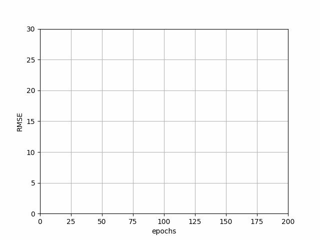
BGD Progression

Mini-Batch Gradient Descent (MBGD)

This algorithm takes a small subset of the given dataset called mini-batch and uses this to calculates the gradient. It's like considering a small amount of population for a survey before taking a step. This balances the speed of SGD and the stability of BGD, making it popular choice for many ML tasks. It is greatly helpful in fine-tuning complex image recognition models.

			# Import required modules
import pandas as pd
import numpy as np
import matplotlib.pyplot as plt
import imageio
import os
plt.grid()
 
def derivative(x, y, m, b): # Function to caluclate derivatives
    m_derivative = -1 * (y - m * x - b) * x
    b_derivative = -1 * (y - m * x - b)
    return m_derivative, b_derivative
 
# Read the data
data = pd.read_csv("data.csv")
 
# Initialize parameters
m = 8
b = 5
learning_rate = 0.06
iterations = 200
n_samples = data.shape[0]
batch_size = 2
 
rmse = [] # List to store RMSE values after each iteration
 
for iter in range(iterations): # Loop to count epochs
 
    sample_num = 0 # Count samples iterated
    
    while sample_num < n_samples: # Loop to iterate through data points
    
        # Initialize Variables to calculate sum of derivatives
        sum_m_grad = 0
        sum_b_grad = 0
 
        # Find the end point of batch
        sample_num_end = min(sample_num + batch_size, n_samples)
    
        while sample_num < sample_num_end: # Loop to iterate through a batch
            m_grad, b_grad = derivative(data["x"][sample_num], data["y"][sample_num], m, b)
            sum_m_grad += m_grad
            sum_b_grad += b_grad
            sample_num += 1
    
        # Calculate Step length
        m_step = learning_rate * sum_m_grad / n_samples
        b_step = learning_rate * sum_b_grad / n_samples
    
        # Update m and b values
        m = m - m_step
        b = b - b_step
 
        # Calculate RMSE Value
    rmse_temp = 0
    for i in range(data.shape[0]):
        rmse_temp += ((data["y"][i] - (m * data["x"][i] + b)) ** 2) ** 0.5
    rmse.append(rmse_temp / data.shape[0])
    
    # Plot RMSE value
    plt.plot(range(1, len(rmse) + 1), rmse, color='red')
    plt.xlim(0, 200)
    plt.ylim(0, 10)
    plt.xlabel('epochs')
    plt.ylabel('RMSE')
    plt.savefig(f"mbgd_graphs/mbgd_{iter}.png")
 
print(f"Achieved values : m = {np.round(m, 2)}, b = {np.round(b, 2)}") # Print achieved values
 
# GIF Generation
images = [imageio.imread(f"mbgd_graphs/mbgd_{x}.png") for x in range(len(os.listdir("mbgd_graphs")))]
imageio.mimsave("mbgd.gif", images)

			# Import required modules
import pandas as pd
import numpy as np
import matplotlib.pyplot as plt
import imageio
import os
plt.grid()
 
def derivative(x, y, m, b): # Function to caluclate derivatives
    m_derivative = -1 * (y - m * x - b) * x
    b_derivative = -1 * (y - m * x - b)
    return m_derivative, b_derivative
 
# Read the data
data = pd.read_csv("data.csv")
 
# Initialize parameters
m = 8
b = 5
learning_rate = 0.06
iterations = 200
n_samples = data.shape[0]
batch_size = 2
 
rmse = [] # List to store RMSE values after each iteration
 
for iter in range(iterations): # Loop to count epochs
 
    sample_num = 0 # Count samples iterated
    
    while sample_num < n_samples: # Loop to iterate through data points
    
        # Initialize Variables to calculate sum of derivatives
        sum_m_grad = 0
        sum_b_grad = 0
 
        # Find the end point of batch
        sample_num_end = min(sample_num + batch_size, n_samples)
    
        while sample_num < sample_num_end: # Loop to iterate through a batch
            m_grad, b_grad = derivative(data["x"][sample_num], data["y"][sample_num], m, b)
            sum_m_grad += m_grad
            sum_b_grad += b_grad
            sample_num += 1
    
        # Calculate Step length
        m_step = learning_rate * sum_m_grad / n_samples
        b_step = learning_rate * sum_b_grad / n_samples
    
        # Update m and b values
        m = m - m_step
        b = b - b_step
 
        # Calculate RMSE Value
    rmse_temp = 0
    for i in range(data.shape[0]):
        rmse_temp += ((data["y"][i] - (m * data["x"][i] + b)) ** 2) ** 0.5
    rmse.append(rmse_temp / data.shape[0])
    
    # Plot RMSE value
    plt.plot(range(1, len(rmse) + 1), rmse, color='red')
    plt.xlim(0, 200)
    plt.ylim(0, 10)
    plt.xlabel('epochs')
    plt.ylabel('RMSE')
    plt.savefig(f"mbgd_graphs/mbgd_{iter}.png")
 
print(f"Achieved values : m = {np.round(m, 2)}, b = {np.round(b, 2)}") # Print achieved values
 
# GIF Generation
images = [imageio.imread(f"mbgd_graphs/mbgd_{x}.png") for x in range(len(os.listdir("mbgd_graphs")))]
imageio.mimsave("mbgd.gif", images)

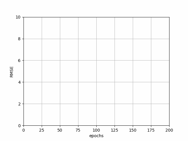
MBGD Progression

Which Variant is most suited for my Application?

Choosing the right variant is very crucial to achieve high accuracies in ML tasks. There are a few key factors to be considered when choosing the variant to be implemented:

Dataset Size: If the dataset is massively huge, SGD's speed shines bright, while BGD might be too slow.
Noise Level: If the dataset is noisy, meaning if there are inconsistencies and values differ significantly, SGD's randomness. Therefore, MBGD or BGD may be preferred.
Model Complexity: Highly complex models may benefit from the smoothness of BGD and MBGD whereas simpler models can tolerate the noisy results of SGD.
Convergence Speed: SGD is much quicker in converging as compared to BGD. But this may also be a negative factor in some applications. MBGD on the other hand can find a sweet spot between SGD and BGD.
Loss Function: The graph of loss function may also influence the selection of a variant. If it is a plain convex with one global minima, SGD may be sufficient but if it is non-convex with multiple local minima, BGD or MBGD may perform better at optimization.

However, it is important to know that there is no "better" variant. As discussed above, each variant has its own perks and weaknesses.

Learning Rate

The learning rate is a crucial parameter in implementing gradient descents for optimization. It essentially controls the pace at which the model updates its internal parameters. Think of it as an accelerator in a car going on a highway. Too less and the car will take a lot of time to reach the exit. Too high and the car will overshoot the exit. In terms of optimization, it decides how long the steps would be. A higher learning rate would make you take big leaps but may also overshoot the optimal point. A low learning rate would require too many iterations or steps. If the learning rate is too high, it is also possible that the optimal point may be overshot all the time and may not be reached.

The Vanishing Gradient

Vanishing gradient is a phenomenon where the gradients become extremely small and this results in slow convergence or impaired learning. This usually happens in deep learning models. A few signs of vanishing gradient problem are:

Slow Training: If the model takes a high amount of time to converge or the improvement in accuracy is little to none, it may be because of vanishing gradient
Inconsistent Layers: If the parameters of one or more layers are impacted significantly less than other layers, that may be the result of vanishing gradient.
Null Weights: The model weights could become zero during training and may not improve again.

To overcome the vanishing gradient problem, certain architectures like Residual Networks (ResNet), Long-Short-Term Memory (LSTM) were introduced. Methods like gradient clipping are also used where the thresholds are set and if the gradient value exceeds the threshold then it is clipped.

Next stop on our journey marks a new beginning! Gear up for the next chapter, where we start working on Machine Learning with a very basic algorithm, the Linear Regression!