So far we have discussed about Linear Regression and Polynomial Regression which help in determining outputs on continuous data. The output of the model in these models can be ranging anywhere from the lower end of the described equation to the upper end. Today we are going to dive into a new category of Machine Learning: Classification.

What is Classification?

The process of mapping the data-points to one or more of the pre-defined classes based on certain statistical evaluations is called Classification. Classification is further divided into three types:

• Binary Classification
• Multi-Class Classification
• Multi-Label Classification

Assume there is a marketing company who is publishing an online advertisement and wants to determine whether or not a user will interact with it or the probability of user interaction. This prediction can be done using ML and the output of the model has to be either Yes or No. This type of problem where there are only two expected labels or outputs are called Binary Classification.

But what if there are more than two expected labels? Let's say a user might want to classify whether an image contains a Dog, a Cat or a Goat. There are three labels in this case. This type of problem is called Multi-Class Classification.

In the above example lies a case where an image may contain more than one animal. Say it has a Dog and a Goat. Here, we are classifying the image to check for multiple classes. This is called Multi-Label Classification.

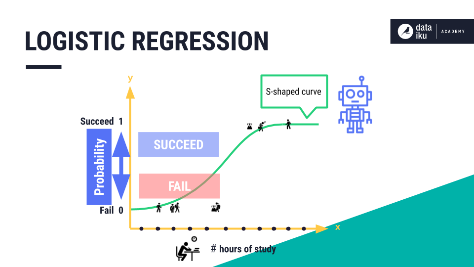
Logistic Regression

In today's article, we will be discussing about Logistic Regression, a Binary Classification algorithm derived from Linear Regression. The Logistic Regression algorithm utilizes the sigmoid function which lines in the range 0 to 1.

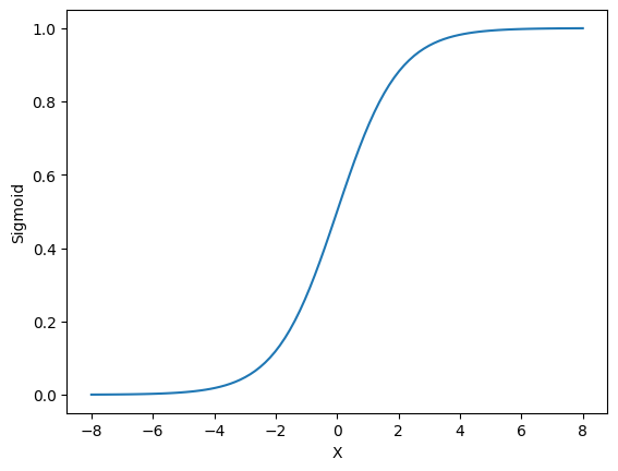
Sigmoid Function

Since the output of the function lies between 0 to 1, there are only two possible outcomes which can be mapped based on the data. For example, 0 can be mapped to "NO" and 1 can be mapped to "YES".

The Logistic Regression algorithm is highly dependent on Linear Regression. The $x$ in sigmoid function uses the same equation as that of Linear Regression i.e. $y = m_1 x_1 + m_2 x_2 + … + b$ and the m and b here are optimized in the training process in order to get the minimum loss. The resulting equation for Logistic Regression is as follows:

Let $z = m_1 x_1 + m_2 x_2 + … + b$

The loss function of Logistic Regression can be defined as:

The Dataset

The above data represents whether or not a specified student passes the exam. Here, the exam result is the label, output or the dependent variable. Hours Studied and Past Score are the features or independent variables. We will be using this data to implement the code for Logistic Regression in Python.

Python Implementation

First off, we import the required modules:

			import numpy as np
import pandas as pd
import math
	

			import numpy as np
import pandas as pd
import math
	

Next step, we load and preprocess the data. This involves converting pass and fail to numeric data i.e. 1 and 0 and then the columns Hours Studied and Past Scores are normalized. Normalization means to scale the values of column between 0 and 1. This is done so that the computation becomes easier and the system can handle larger values. The formula for normalization is:

			# Load the data
data = pd.read_csv("data.csv")
 
# Convert "Pass" and "Fail" to 1 and 0 respectively
data["Exam Result Numeric"] = data["Exam Result"].apply(lambda x : 0 if x == "Fail" else 1)
 
# Normalization of data
max_val = [max(data["Hours Studied"]), max(data["Past Score"])]
min_val = [min(data["Hours Studied"]), min(data["Past Score"])]
data["Hours Studied"] = (data["Hours Studied"] - min_val[0]) / (max_val[0] - min_val[0])
data["Past Score"] = (data["Past Score"] - min_val[1]) / (max_val[1] - min_val[1])
 
# Separating Features and Label as x and y
x = data[["Hours Studied", "Past Score"]].to_numpy()
y = data['Exam Result Numeric'].to_numpy()
n = len(y)
	

			# Load the data
data = pd.read_csv("data.csv")
 
# Convert "Pass" and "Fail" to 1 and 0 respectively
data["Exam Result Numeric"] = data["Exam Result"].apply(lambda x : 0 if x == "Fail" else 1)
 
# Normalization of data
max_val = [max(data["Hours Studied"]), max(data["Past Score"])]
min_val = [min(data["Hours Studied"]), min(data["Past Score"])]
data["Hours Studied"] = (data["Hours Studied"] - min_val[0]) / (max_val[0] - min_val[0])
data["Past Score"] = (data["Past Score"] - min_val[1]) / (max_val[1] - min_val[1])
 
# Separating Features and Label as x and y
x = data[["Hours Studied", "Past Score"]].to_numpy()
y = data['Exam Result Numeric'].to_numpy()
n = len(y)
	

Now we need to initialize the model parameters and then we go ahead and train the logistic regression model. Refer the code below:

			# Initialization of model parameters
m1 = np.random.uniform(-5, 5)
m2 = np.random.uniform(-5, 5)
b = np.random.uniform(-5, 5)
learning_rate = 0.5
iterations = 200
 
# Loop to count epochs
for _ in range(iterations):
    
    # Loop to iterate through each sample
    for i in range(n):
 
        # Calculate z
        z = m1 * x[i][0] + m2 * x[i][1] + b
 
        # Calculate sigmoid function
        if z < 0:
            y_pred = 1 - 1 / (1 + math.exp(z))
        else:
            y_pred = 1 / (1 + math.exp(-z))
 
        # Calculate the loss
        log_loss = y[i] * math.log(y_pred) - (1 - y[i]) * math.log(1 - y_pred)
        
        # Calculate Gradient
        m1_grad = log_loss * x[i][0]
        m2_grad = log_loss * x[i][1]
        b_grad = log_loss
 
        # Calculate Step-Length
        m1_step = learning_rate * m1_grad
        m2_step = learning_rate * m2_grad
        b_step = learning_rate * b_grad
 
        # Update Model Parameters
        m1 -= m1_step
        m2 -= m2_step
        b -= b_step
	

			# Initialization of model parameters
m1 = np.random.uniform(-5, 5)
m2 = np.random.uniform(-5, 5)
b = np.random.uniform(-5, 5)
learning_rate = 0.5
iterations = 200
 
# Loop to count epochs
for _ in range(iterations):
    
    # Loop to iterate through each sample
    for i in range(n):
 
        # Calculate z
        z = m1 * x[i][0] + m2 * x[i][1] + b
 
        # Calculate sigmoid function
        if z < 0:
            y_pred = 1 - 1 / (1 + math.exp(z))
        else:
            y_pred = 1 / (1 + math.exp(-z))
 
        # Calculate the loss
        log_loss = y[i] * math.log(y_pred) - (1 - y[i]) * math.log(1 - y_pred)
        
        # Calculate Gradient
        m1_grad = log_loss * x[i][0]
        m2_grad = log_loss * x[i][1]
        b_grad = log_loss
 
        # Calculate Step-Length
        m1_step = learning_rate * m1_grad
        m2_step = learning_rate * m2_grad
        b_step = learning_rate * b_grad
 
        # Update Model Parameters
        m1 -= m1_step
        m2 -= m2_step
        b -= b_step
	

This finishes our model training. Let's check out the outputs for each sample in our dataset.

			# Calculate model output for every sample
preds = [1/(1 + math.exp(-(m1*i[0] + m2*i[1] + b))) for i in x]
 
# Map 0 to Fail and 1 to Pass
preds = list(map(lambda x: "Pass" if x > 0.4 else "Fail", preds))
 
# Add the predictions to DataFrame
data["Predictions"] = preds
	

			# Calculate model output for every sample
preds = [1/(1 + math.exp(-(m1*i[0] + m2*i[1] + b))) for i in x]
 
# Map 0 to Fail and 1 to Pass
preds = list(map(lambda x: "Pass" if x > 0.4 else "Fail", preds))
 
# Add the predictions to DataFrame
data["Predictions"] = preds
	

Evaluation for Classification Model

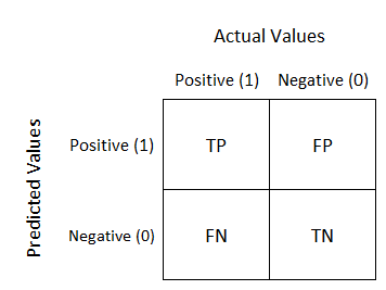
There are several ways to evaluate a Classification Model. Before we dive into them, Let's discuss a few general terms which must be known in order to understand them.

True Positives (TP) - Number of correctly predicted positive samples.

True Negatives (TN) - Number of correctly predicted negative samples.

False Positives (FP) - Number of samples for which model predicted positive but actual output is negative

False Negative (FN) - Number of samples for which model predicted negative but actual output is positive

Just to make it more clear, let's see this on a table.

Now let's discuss the evaluation metrics.

Accuracy

Accuracy is defined as the percentage of samples correctly prediction with respect to total number of samples.

			actual_outputs = data["Exam Result"]
predicted_outputs = data["Predictions"]
 
correctly_predicted = 0
for actual, predicted in zip(actual_outputs, predicted_outputs):
    if actual == predicted:
        correctly_predicted += 1
accuracy = correctly_predicted / len(actual_outputs)
print(accuracy)
	

			actual_outputs = data["Exam Result"]
predicted_outputs = data["Predictions"]
 
correctly_predicted = 0
for actual, predicted in zip(actual_outputs, predicted_outputs):
    if actual == predicted:
        correctly_predicted += 1
accuracy = correctly_predicted / len(actual_outputs)
print(accuracy)
	

			1.0
	

			1.0
	

Classification Matrix

A classification matrix is a matrix representation of the categories that we discussed above. The TP, FP, TN and FN. These values are arranged in the following form:

Sample Confusion Matrix

Let's generate a confusion matrix for our code using the scikit-learn library in python.

			from sklearn.metrics import confusion_matrix, ConfusionMatrixDisplay
import matplotlib.pyplot as plt
 
cm = confusion_matrix(actual_outputs, predicted_outputs)
 
tp = cm[0][0]
fp = cm[0][1]
fn = cm[1][0]
tn = cm[1][1]
 
cm_display = ConfusionMatrixDisplay(cm)
cm_display.plot()
	

			from sklearn.metrics import confusion_matrix, ConfusionMatrixDisplay
import matplotlib.pyplot as plt
 
cm = confusion_matrix(actual_outputs, predicted_outputs)
 
tp = cm[0][0]
fp = cm[0][1]
fn = cm[1][0]
tn = cm[1][1]
 
cm_display = ConfusionMatrixDisplay(cm)
cm_display.plot()
	

The output image of the above code is:

Generated Confusion Matrix

In the code for confusion matrix, we have saved the tp, fp, tn, fn in variables. These variables can be further used to calculate more metrics. Let's look at those.

Precision

Precision is defined as the quality of a positive prediction made by the model, i.e., the percentage of True Positive predictions as compared to total number of positive predictions.

			precision = tp / (fp + tp)
print(precision)
	

			precision = tp / (fp + tp)
print(precision)
	

			1.0
	

			1.0
	

Recall

It is defined as the percentage of correctly identified positive samples as compared to the total number of positive samples in the original dataset.

			recall = tp / (tp + fn)
print(recall)
	

			recall = tp / (tp + fn)
print(recall)
	

			1.0
	

			1.0
	

F1 Score

The F1 Score is the combination of both Precision and Recall and provides a single metric to understand model performance. The equation for F1 Score is:

			f1score = 2 * tp / (2 * tp + fp + fn)
print(f1score)
	

			f1score = 2 * tp / (2 * tp + fp + fn)
print(f1score)
	

			1.0
	

			1.0
	

The above discussed are some most frequently used evaluation methods for classification problems.

Up Next: We are going to talk about a new algorithm: The Decision Tree. Stay tuned, stay focused and don't forget to share if you find this helpful!