What is Polynomial Regression?

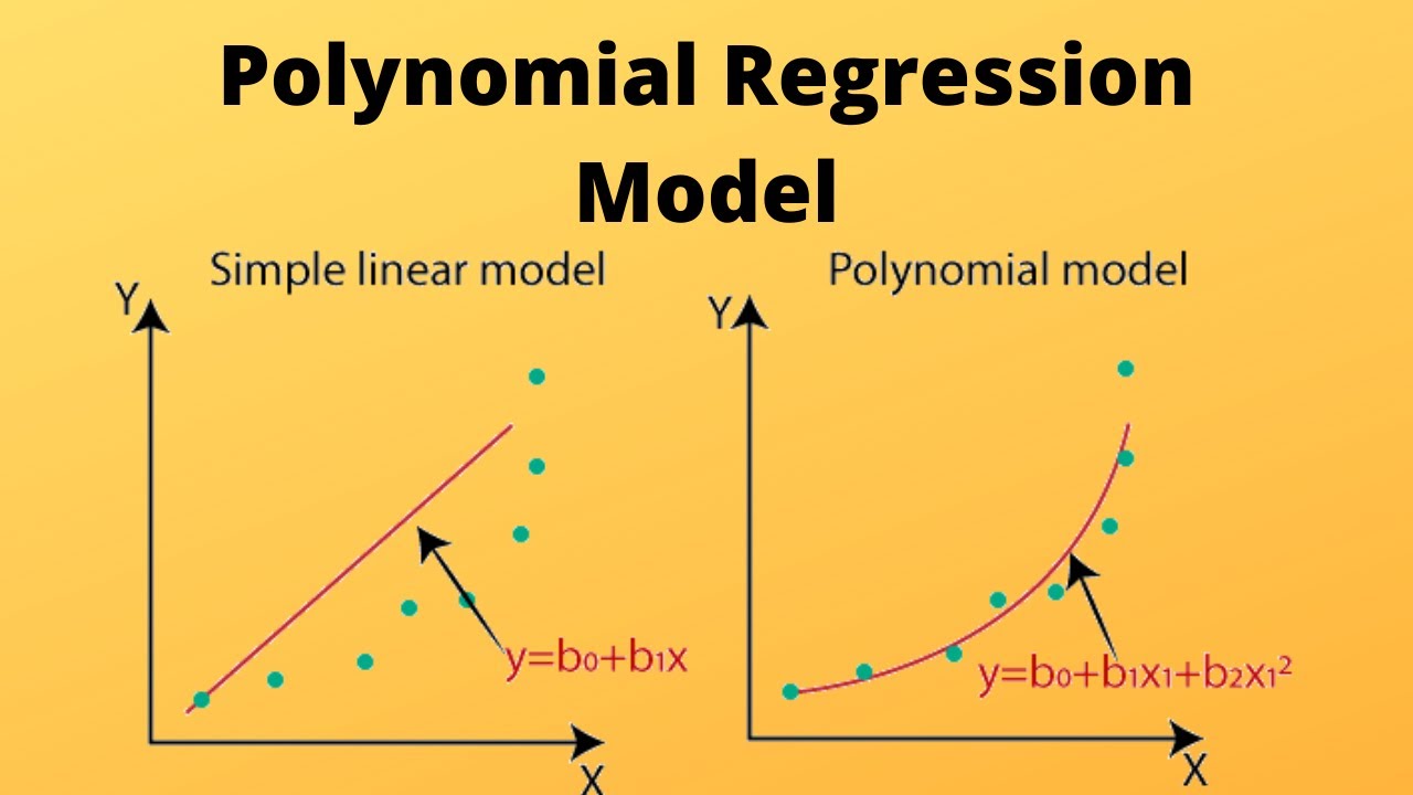
Polynomial regression is a statistical method that extends linear regression to model nonlinear relationships between variables. It achieves this by fitting a polynomial equation, rather than a straight line, to the data. It fits curves to data by raising the independent variable to various powers, capturing nonlinear relationships between the independent and dependent variables.

In polynomial regression, the relationship between the independent variable $x$ and the dependent variable $y$ is modeled as a curve, rather than a straight line. This allows for capturing more complex, nonlinear relationships that simple linear regression cannot. Here, Instead of a straight line, we use a polynomial equation of degree n:

Where:

• $y$ : The dependent variable (predicted value)
• $x$ : The independent variable
• $eta_0$, $eta_1$ , $eta_2$ , …, $eta_n$ : Coefficients representing the influence of each power of x
• $n$ : Degree of the polynomial (highest power of x)
• $arepsilon$ : Random error term

The values of $eta_0$, $eta_1$ , $eta_2$ , …, $eta_n$ and $arepsilon$ are determined during the training phase of the model. We Use the least squares method to estimate the coefficients $eta_0$, $eta_1$ , $eta_2$ , …, $eta_n$ using the given variables in the data which are $x$ and $y$ that minimize the sum of squared residuals (differences between predicted and actual y values).

The value of $n$ determines the degree and shape of the curve, i.e., whether its a straight line, parabolic, or more complex shapes. The random error term ($arepsilon$) in the polynomial regression equation represents the unexplained portion of the dependent variable ($y$). It accounts for all the factors influencing $y$ that are not included in the polynomial model itself. In essence, it reflects the inherent noise and variability in the data that cannot be captured by the fitted curve.

Types of Polynomial Regression

we can broadly classify the types of polynomial regression based on degree of the polynomial ($n$) :

• Linear degree ($n$ = 1): Equivalent to simple linear regression which involves only one independent variable. The relationship between the independent variable $x$ and the dependent variable $y$ is modeled as straight line.

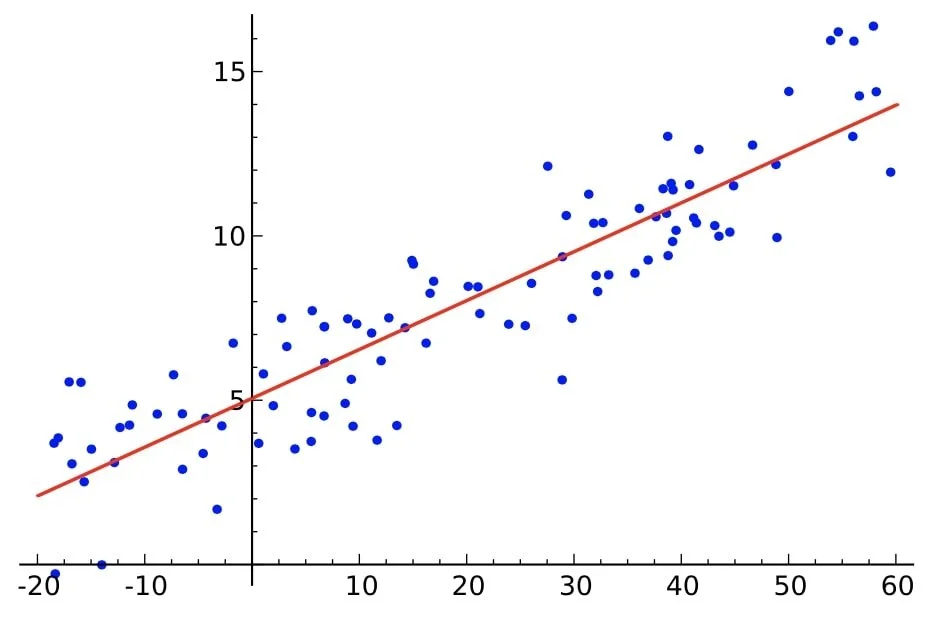
Linear Regression

• Higher degrees ($n$ > 1): Allow for modeling curves, such as:
• Quadratic ($n$ = 2): This is an extension of simple linear regression where the degree of the equation is 2 and we find the equation values of the parabola that best fits a set of data. The parabola will be either concave down or concave up.

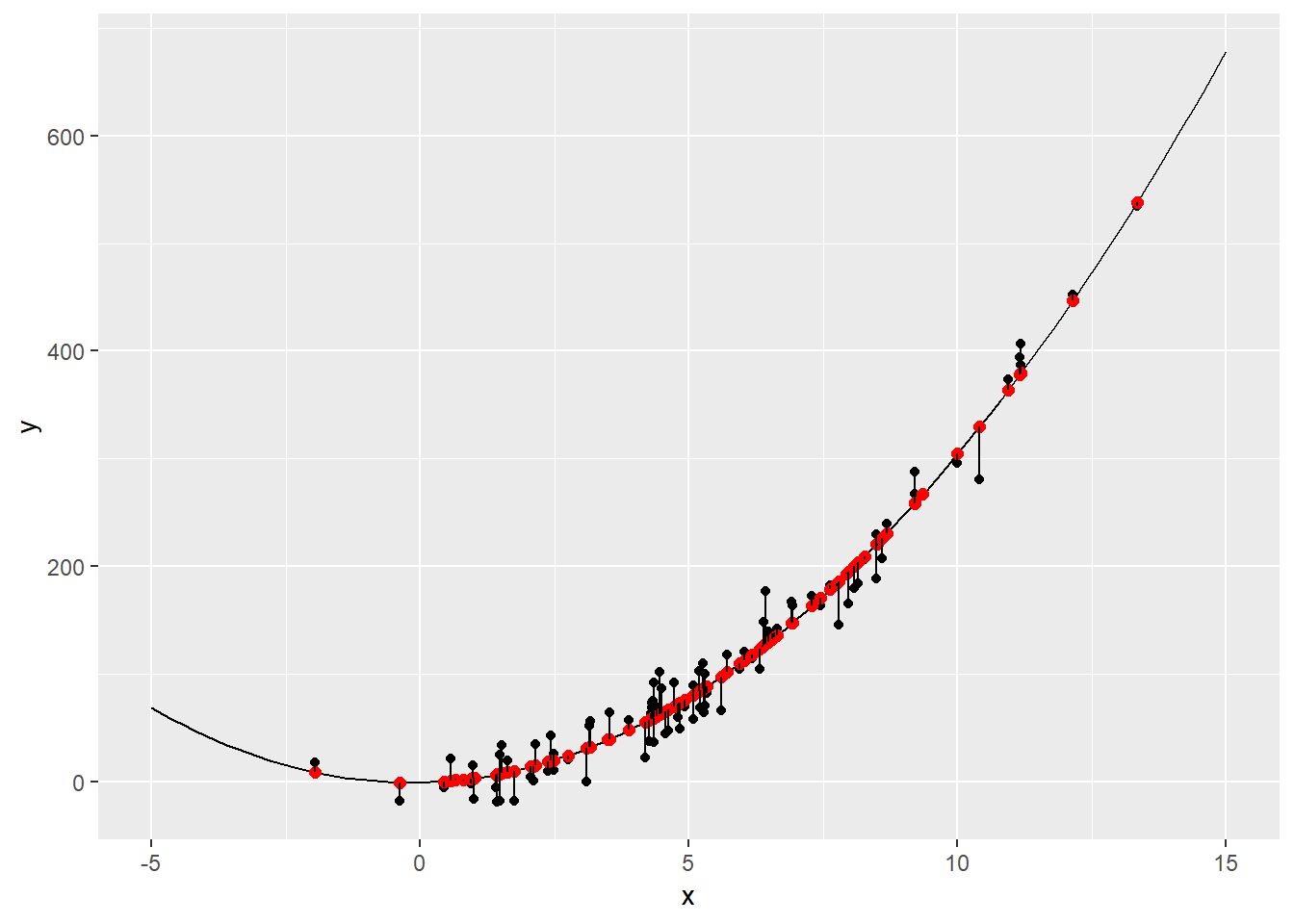
Quadratic Polynomial Regression

• Cubic ($n$ = 3): This regression technique has the degree of equation as 3 and we find the equation values of the shaped curve that best fits the given data. The graph is usually in the shape of "S" which will be passing through or near to most of the data points.

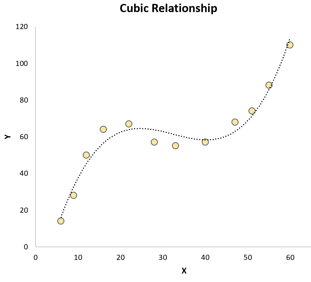
Cubic Polynomial Regression

• Quartic ($n$ = 4): This regression technique has the degree of equation as 4 which is the highest order polynomial equation and we find the equation of the complex shaped curve which passes through all the scattered data points. The graph is usually in the shape of "W" which may be inverted at times.

Quartic Polynomial Regression

Each of the above mentioned type is used according to the pattern the data points show when plotted on a scatter plot. The error will be reduced and the predictions will be accurate is the proper polynomial degree regression is used.

Math behind Polynomial Regression

The mathematics involved in polynomial regression remains pretty much same as the linear regression one, where we calculate the sum of mean squared error for all the data points.

Hypothesis Function:

In polynomial regression, the hypothesis function is no longer a simple linear equation. Instead, it's a polynomial of a chosen degree $n$. Here's the general form:

where:

• $h(x)$ is the predicted value of the dependent variable y for a given input value x.
• $\theta_i$ are the coefficients of the polynomial, to be determined through the learning process.
• $n$ is the degree of the polynomial.

Cost Function:

Similar to linear regression, we use a cost function to measure how well the hypothesis function fits the training data. The most common cost function in polynomial regression is still the mean squared error (MSE) $$[Error = (predicted - actual)^2]$$ :

where:

• $J(\theta)$ is the cost function value.
• $m$ is the number of data points.
• $h(x_i)$ is the predicted value for the $i$-th data point.
• $y_i$ is the actual value of the $i$-th data point.

Gradient Descent:

We use gradient descent to minimize the cost function and find the optimal values for the polynomial coefficients ($\theta_j$). The update rule for each coefficient is similar to linear regression, but with additional terms due to the higher degree of the polynomial:

where:

• $alpha$ is the learning rate.
• $j$ iterates over all coefficients (0 to $n$).

We repeat the above process until the cost converges to a minimum. Once we have the optimized parameters $\theta_j$, we use the hypothesis function to make predictions for upcoming values.

Python Implementation

Let's import the required python modules:

			import numpy as np
import matplotlib.pyplot as plt
import pandas as pd
from sklearn.model_selection import train_test_split
from sklearn.metrics import mean_absolute_error, mean_squared_error, r2_score
import imageio
import os
	

			import numpy as np
import matplotlib.pyplot as plt
import pandas as pd
from sklearn.model_selection import train_test_split
from sklearn.metrics import mean_absolute_error, mean_squared_error, r2_score
import imageio
import os
	

Quadratic polynomial regression using BGD

We will be implementing the quadratic polynomial regression for the equation $y=2x^2+5x-3$ using the below defined functions:

			def predict_quadratic(x, theta):
    return theta[0] + theta[1] * x + theta[2] * x**2
 
def quadratic_regression_gradient_descent(x, y, learning_rate=0.01, num_iterations=100):
 
    m = len(x)  # Number of data points
 
    # Initialize coefficients randomly
    theta = np.random.randn(3)
 
    for iter in range(num_iterations):
        # Hypothesis function
        h = theta[0] + theta[1] * x + theta[2] * x**2
 
        # Cost function (MSE)
        cost = (1/(2*m)) * np.sum((h - y)**2)
 
        # Gradients for each coefficient
        grad_0 = (1/m) * np.sum(h - y)
        grad_1 = (1/m) * np.sum((h - y) * x)
        grad_2 = (1/m) * np.sum((h - y) * x**2)
 
        # Update coefficients using gradient descent
        theta[0] -= learning_rate * grad_0
        theta[1] -= learning_rate * grad_1
        theta[2] -= learning_rate * grad_2
 
        fig = plt.figure(figsize=(8, 6))
        plt.scatter(x, y, label='Data Point', color='Green')
        plt.plot(x, [predict_quadratic(i, theta) for i in x], label='Quadratic Regression Line', color='Red')
        plt.xlabel('x')
        plt.ylabel('y')
        plt.title('Quadratic Polynomial Regression')
        plt.legend()
        plt.grid(linestyle = '--', linewidth = 0.5)
        plt.savefig(f"quadpoly_graphs/quadpoly_{iter}.png")
        plt.close(fig)
 
    return theta
 
# Generate sample data with a quadratic relationship
x = np.linspace(-3, 3, 100)
y = 2 * x**2 + 5 * x - 3 + np.random.randn(100) * 2  # Add some noise
 
X_train, X_test, y_train, y_test = train_test_split(x, y, test_size=0.2, random_state=42, shuffle=True)
 
Finaltheta = quadratic_regression_gradient_descent(X_train,y_train)
 
y_pred = predict_quadratic(X_test, Finaltheta)
 
images = [imageio.imread(f"quadpoly_graphs/quadpoly_{i}.png") for i in range(len(os.listdir("quadpoly_graphs")))]
imageio.mimsave("quadpoly.gif", images)
	

			def predict_quadratic(x, theta):
    return theta[0] + theta[1] * x + theta[2] * x**2
 
def quadratic_regression_gradient_descent(x, y, learning_rate=0.01, num_iterations=100):
 
    m = len(x)  # Number of data points
 
    # Initialize coefficients randomly
    theta = np.random.randn(3)
 
    for iter in range(num_iterations):
        # Hypothesis function
        h = theta[0] + theta[1] * x + theta[2] * x**2
 
        # Cost function (MSE)
        cost = (1/(2*m)) * np.sum((h - y)**2)
 
        # Gradients for each coefficient
        grad_0 = (1/m) * np.sum(h - y)
        grad_1 = (1/m) * np.sum((h - y) * x)
        grad_2 = (1/m) * np.sum((h - y) * x**2)
 
        # Update coefficients using gradient descent
        theta[0] -= learning_rate * grad_0
        theta[1] -= learning_rate * grad_1
        theta[2] -= learning_rate * grad_2
 
        fig = plt.figure(figsize=(8, 6))
        plt.scatter(x, y, label='Data Point', color='Green')
        plt.plot(x, [predict_quadratic(i, theta) for i in x], label='Quadratic Regression Line', color='Red')
        plt.xlabel('x')
        plt.ylabel('y')
        plt.title('Quadratic Polynomial Regression')
        plt.legend()
        plt.grid(linestyle = '--', linewidth = 0.5)
        plt.savefig(f"quadpoly_graphs/quadpoly_{iter}.png")
        plt.close(fig)
 
    return theta
 
# Generate sample data with a quadratic relationship
x = np.linspace(-3, 3, 100)
y = 2 * x**2 + 5 * x - 3 + np.random.randn(100) * 2  # Add some noise
 
X_train, X_test, y_train, y_test = train_test_split(x, y, test_size=0.2, random_state=42, shuffle=True)
 
Finaltheta = quadratic_regression_gradient_descent(X_train,y_train)
 
y_pred = predict_quadratic(X_test, Finaltheta)
 
images = [imageio.imread(f"quadpoly_graphs/quadpoly_{i}.png") for i in range(len(os.listdir("quadpoly_graphs")))]
imageio.mimsave("quadpoly.gif", images)
	

The Representation of the training process and curve fitting is depicted by the following illustration:

Quadratic Polynomial Regression Graph

The error calculation for the quadratic polynomial regression can be done through the following code snippet:

			mae = mean_absolute_error(y_test, y_pred)
mse = mean_squared_error(y_test, y_pred)
rmse = np.sqrt(mse)
r_squared = r2_score(y_test, y_pred)
 
# Print the error metrics
print("Mean Absolute Error (MAE):", mae)
print("Mean Squared Error (MSE):", mse)
print("Root Mean Squared Error (RMSE):", rmse)
print("R-squared (R2):", r_squared)
	

			mae = mean_absolute_error(y_test, y_pred)
mse = mean_squared_error(y_test, y_pred)
rmse = np.sqrt(mse)
r_squared = r2_score(y_test, y_pred)
 
# Print the error metrics
print("Mean Absolute Error (MAE):", mae)
print("Mean Squared Error (MSE):", mse)
print("Root Mean Squared Error (RMSE):", rmse)
print("R-squared (R2):", r_squared)
	

			Mean Absolute Error (MAE): 2.257098279170521
Mean Squared Error (MSE): 8.113227442967567
Root Mean Squared Error (RMSE): 2.848372771069048
R-squared (R2): 0.8989093949486041
	

			Mean Absolute Error (MAE): 2.257098279170521
Mean Squared Error (MSE): 8.113227442967567
Root Mean Squared Error (RMSE): 2.848372771069048
R-squared (R2): 0.8989093949486041
	

Cubic Polynomial Regression

We will be implementing the quadratic polynomial regression for the equation $y=2x^3+5x^2-3$ using the below defined functions:

			def predict_cubic(x, theta):
 
    return theta[0] + theta[1] * x + theta[2] * x**2 + theta[3] * x**3
 
def cubic_regression_gradient_descent(x, y, learning_rate=0.01, num_iterations=100):
 
    m = len(x)  # Number of data points
 
    # Initialize coefficients randomly (now with 4 for cubic)
    theta = np.random.randn(4)
 
    for iter in range(num_iterations):
        # Hypothesis function (now includes x**3 term)
        h = theta[0] + theta[1] * x + theta[2] * x**2 + theta[3] * x**3
 
        # Cost function (MSE)
        cost = (1/(2*m)) * np.sum((h - y)**2)
 
        # Gradients for each coefficient (including gradient for theta[3])
        grad_0 = (1/m) * np.sum(h - y)
        grad_1 = (1/m) * np.sum((h - y) * x)
        grad_2 = (1/m) * np.sum((h - y) * x**2)
        grad_3 = (1/m) * np.sum((h - y) * x**3)
 
        # Update coefficients using gradient descent
        theta[0] -= learning_rate * grad_0
        theta[1] -= learning_rate * grad_1
        theta[2] -= learning_rate * grad_2
        theta[3] -= learning_rate * grad_3
 
        fig = plt.figure(figsize=(8, 6))
        plt.scatter(x, y, label='Data Point', color='Green')
        plt.plot(x, [predict_cubic(i, theta) for i in x], label='Cubic Regression Line', color='Red')
        plt.xlabel('x')
        plt.ylabel('y')
        plt.title('Cubic Polynomial Regression')
        plt.legend()
        plt.grid(linestyle = '--', linewidth = 0.5)
        plt.savefig(f"cubepoly_graphs/cubepoly_{iter}.png")
        plt.close(fig)
 
    return theta
 
# Generate sample data with a Cubic relationship
x = np.linspace(-3, 3, 100)
y = 2 * x**3 + 5 * x**2 - 3 + np.random.randn(100) * 2
 
X_train, X_test, y_train, y_test = train_test_split(x, y, test_size=0.2, random_state=42, shuffle=True)
 
Finaltheta = cubic_regression_gradient_descent(X_train,y_train)
 
y_pred = predict_cubic(X_test, Finaltheta)
 
images = [imageio.imread(f"cubepoly_graphs/cubepoly_{i}.png") for i in range(len(os.listdir("cubepoly_graphs")))]
imageio.mimsave("cubepoly.gif", images)
	

			def predict_cubic(x, theta):
 
    return theta[0] + theta[1] * x + theta[2] * x**2 + theta[3] * x**3
 
def cubic_regression_gradient_descent(x, y, learning_rate=0.01, num_iterations=100):
 
    m = len(x)  # Number of data points
 
    # Initialize coefficients randomly (now with 4 for cubic)
    theta = np.random.randn(4)
 
    for iter in range(num_iterations):
        # Hypothesis function (now includes x**3 term)
        h = theta[0] + theta[1] * x + theta[2] * x**2 + theta[3] * x**3
 
        # Cost function (MSE)
        cost = (1/(2*m)) * np.sum((h - y)**2)
 
        # Gradients for each coefficient (including gradient for theta[3])
        grad_0 = (1/m) * np.sum(h - y)
        grad_1 = (1/m) * np.sum((h - y) * x)
        grad_2 = (1/m) * np.sum((h - y) * x**2)
        grad_3 = (1/m) * np.sum((h - y) * x**3)
 
        # Update coefficients using gradient descent
        theta[0] -= learning_rate * grad_0
        theta[1] -= learning_rate * grad_1
        theta[2] -= learning_rate * grad_2
        theta[3] -= learning_rate * grad_3
 
        fig = plt.figure(figsize=(8, 6))
        plt.scatter(x, y, label='Data Point', color='Green')
        plt.plot(x, [predict_cubic(i, theta) for i in x], label='Cubic Regression Line', color='Red')
        plt.xlabel('x')
        plt.ylabel('y')
        plt.title('Cubic Polynomial Regression')
        plt.legend()
        plt.grid(linestyle = '--', linewidth = 0.5)
        plt.savefig(f"cubepoly_graphs/cubepoly_{iter}.png")
        plt.close(fig)
 
    return theta
 
# Generate sample data with a Cubic relationship
x = np.linspace(-3, 3, 100)
y = 2 * x**3 + 5 * x**2 - 3 + np.random.randn(100) * 2
 
X_train, X_test, y_train, y_test = train_test_split(x, y, test_size=0.2, random_state=42, shuffle=True)
 
Finaltheta = cubic_regression_gradient_descent(X_train,y_train)
 
y_pred = predict_cubic(X_test, Finaltheta)
 
images = [imageio.imread(f"cubepoly_graphs/cubepoly_{i}.png") for i in range(len(os.listdir("cubepoly_graphs")))]
imageio.mimsave("cubepoly.gif", images)
	

The Representation of the training process and curve fitting is depicted by the following illustration:

Cubic Polynomial Regression Graph

The error calculation for the cubic polynomial regression can be done through the following code snippet:

			mae = mean_absolute_error(y_test, y_pred)
mse = mean_squared_error(y_test, y_pred)
rmse = np.sqrt(mse)
r_squared = r2_score(y_test, y_pred)
 
# Print the error metrics
print("Mean Absolute Error (MAE):", mae)
print("Mean Squared Error (MSE):", mse)
print("Root Mean Squared Error (RMSE):", rmse)
print("R-squared (R2):", r_squared)
	

			mae = mean_absolute_error(y_test, y_pred)
mse = mean_squared_error(y_test, y_pred)
rmse = np.sqrt(mse)
r_squared = r2_score(y_test, y_pred)
 
# Print the error metrics
print("Mean Absolute Error (MAE):", mae)
print("Mean Squared Error (MSE):", mse)
print("Root Mean Squared Error (RMSE):", rmse)
print("R-squared (R2):", r_squared)
	

			Mean Absolute Error (MAE): 2.370609761677744
Mean Squared Error (MSE): 7.706860468026003
Root Mean Squared Error (RMSE): 2.776123280408491
R-squared (R2): 0.9689277933130518
	

			Mean Absolute Error (MAE): 2.370609761677744
Mean Squared Error (MSE): 7.706860468026003
Root Mean Squared Error (RMSE): 2.776123280408491
R-squared (R2): 0.9689277933130518
	

The error metrics for both the models define how accurate the model is predicting the dependent values $y$ from the independent values $x$

That's all about linear and polynomial regression. Hold onto your hats, because in our next post, we're diving into the world of classification through logistic regression algorithm!